Columnar Data : how it works
We’re probably all fairly familiar now with BLU acceleration and the advantages of storing analytical data in a columnar format. If not, and by way of a recap; what we can now do is return much smaller results sets to our analytical queries, in a highly-compressed format, thereby reducing I/O and maximizing usage of our memory resources.
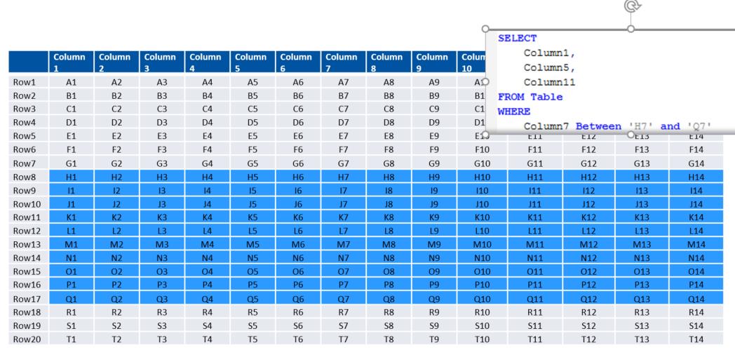
If you think of data stored in a conventional row-based format (and I apologize to anyone at IDUG 2017 who has already sat through this material in my Db2 V11.1 Hits and Misses presentation), and a simple query to run against it, like the one below, you will be retrieving an ‘area’ of data like this (click image to enlarge)
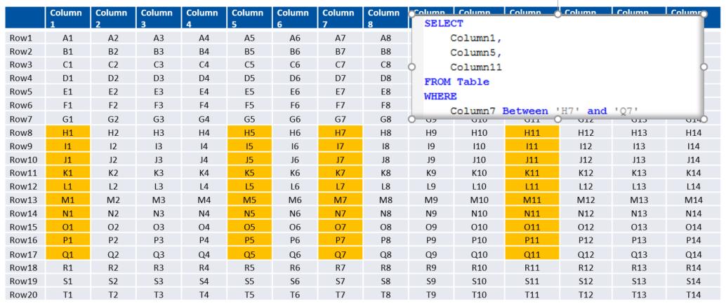
If you were doing the same thing with your data stored in a columnar fashion, the footprint of your result set would be reduced to this
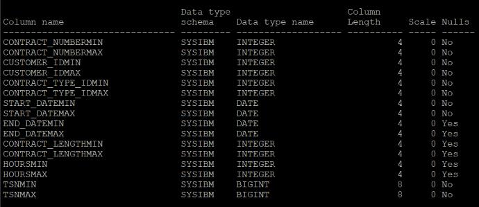
This is achieved through not only the storage of data in columns, but the technique of ‘data-skipping’, where a synopsis table is automatically stored (and automatically maintained) with the minimum and maximum values for each column stored, for every 512 rows. So, my main fact table; CONTRACT, looks like this
And the associated synopsis table looks like this
If I had to find just the data where the HOURS value was less than 298, what Db2 would be doing ‘under-the-covers’ would be to examine the contents of the synopsis table to find just the qualifying TSN (Tuple Sequence Numbers); essentially finding the blocks of data that will contain just these values and allowing Db2 to extract just those columns we need for these corresponding ranges. You can check it yourself as the synopsis table is just another table, albeit one over which you have no control:
You can see here that using the Synopsis table has identified 2 blocks of data; each of 1,023 tuples. That’s eliminating a significant volume of data from the query, considering there are 5,000,000 unique values in this table.
Add into this mix that we have some pretty aggressive compression with columnar data, and the result set footprint becomes even smaller (see PCTPAGESSAVED in SYSCAT.TABLES for an estimate of how much space is saved compared to a row-based version of the same data). In this case, my CONTRACT table is showing a figure of 45%. And remember that this columnar data will stay compressed once it’s read into memory and whilst the query operates against it.
So, this is all good stuff; terrific performance benefits to be had without any intervention from you, the DBA. It comes straight out of the box.
The CTQ boundary : V11
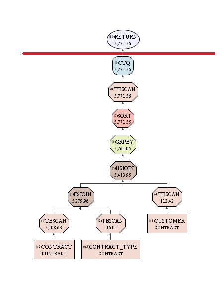
And when you explain your queries you can see how much of the processing is going to take place in columnar format. At some point the data needs to be converted to the familiar row-based result set, so that your users and applications can actually read it and that is shown in your access path with a CTQ (Columnar Table Queue) operator.
Everything below that CTQ operator is taking advantage of the columnar data storage, the data skipping processing, the actionable compression and delivering performance benefits to your analytical queries. With V11 you can now process further OLAP functions, sorts and Nested Loop Joins on columnar data; further leveraging the performance benefits.
But notice the other thing about this access path; the retrieval of data from the tables just appears as a Table Scan (TBSCAN); there’s no indication of if, or how efficiently, the synopsis tables are used. You can’t see what Index Usage there is; even though you can only create UNIQUE Indexes on Columnar Tables, there are other automatically created (and maintained) indexes. For each columnar table (including the Synopsis table) there will be a CPMA (Columnar Page Map) index which operates a bit like the Block Index of a Multi-Dimensional Cluster. But the explain won’t show if, or how well, this is being exploited either.
And this leads us to the crux of the matter; what can we do to explore how well the columnar operations are being exercised? I’ll take a look at some of the options in the next blog.


